Two-dimensional spectral analysis
Contents
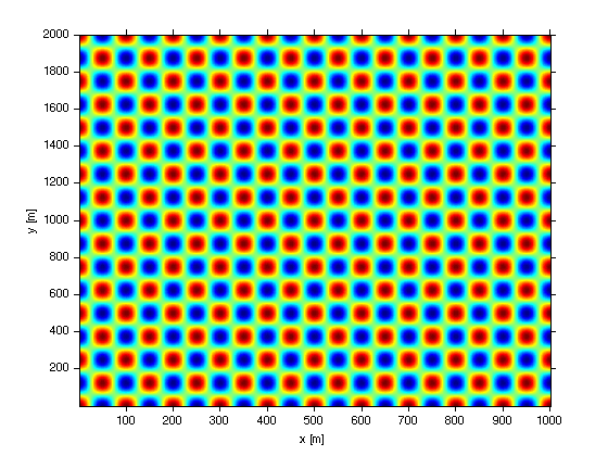
Make a synthesized 2-D signal
Here, let  $ and
$ and  $ be the space the data occupies, and
  $ be the signal.
xx = 1:1000;
yy = 1:2000;

[x,y]=meshgrid(xx,yy);

kx0 = 0.01;
ky0 = 0.004;

w = cos(x*2*pi*kx0).*cos(y*2*pi*ky0);

figure(1);clf
imagesc(xx,yy,w);
set(gca,'ydir','no');
xlabel('x [m]');
ylabel('y [m]');
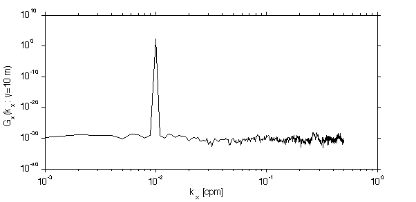
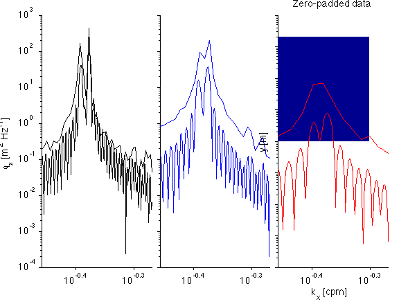
Lets take the powerspectrum in x and look at it...
% first k_x = [0:N-1]/\deltax

M = length(xx);
N = length(yy);

dx = 1;
k_x = (0:M-1)/dx/M;
dy = 1;
k_y = (0:N-1)/dx/N;


X = fft(w')';

Gx = (1/M/dx)*X(:,2:M/2).* conj(X(:,2:M/2));
k_x = k_x(2:M/2);
The spectrum of any individual row is just the spectrum of w at that value of y: For this example, it is just a spike at
 $.
$.
figure(2);clf

loglog(k_x,Gx(10,:))
xlabel('k_x [cpm]');
ylabel('G_x(k_x: y=10 m)');
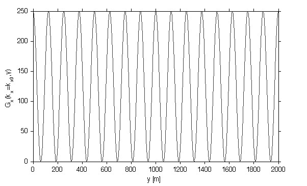
The value of this peak varies with y as  $.
$.
in = find(k_x>kx0);
in = in(1)-1;
figure(3); clf;
plot(y,Gx(:,in));
xlabel('y [m]');
ylabel('G_x(k_x=k_{x0},y)');
or visualized in 2-D....
figure(4);

pcolor(k_x,yy,real(Gx));shading flat;
set(gca,'xscale','log');
xlabel('k_x [cpm]');
ylabel('y [m]');
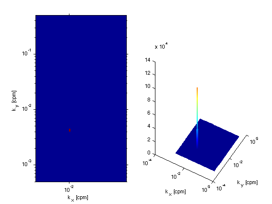
Taking the 2-D Power Spectrum....
XY = fft(fft(w')');
k_x = (0:M-1)/dx/M;
k_y = (0:N-1)/dx/N;

GXY = (1/M/dx)*(1/N/dy)*XY(2:N/2,2:M/2).* conj(XY(2:N/2,2:M/2));
k_y = k_y(2:N/2);
k_x = k_x(2:M/2);
We see the result is a single peak at  $
$
figure(5);clf
subplot(1,2,1);

pcolor(k_x,k_y,real(GXY));shading flat;
set(gca,'xscale','log','yscale','log')
xlabel('k_x [cpm]');
ylabel('k_y [cpm]');

subplot(1,2,2);

surface(k_x,k_y,real(GXY));shading interp;
set(gca,'xscale','log','yscale','log')
xlabel('k_x [cpm]');
ylabel('k_y [cpm]');
view(30,30);

w0 = w;
A more interesting process.
Consider a 2-D white noise process, and then integrate separately in both x and y to get red processes in both dimensions.. Then ad the noise back on...
wp = randn(N,M);
w = cumsum(cumsum(wp)')';
w = w+wp*50+1000*w0;


figure(10);clf
subplot(2,1,1);

imagesc(xx,yy,wp);
set(gca,'ydir','nor');
title('w''');
ylabel('y [m]');

subplot(2,1,2);

imagesc(xx,yy,w);
title('w');
set(gca,'ydir','nor');
xlabel('x [m]');

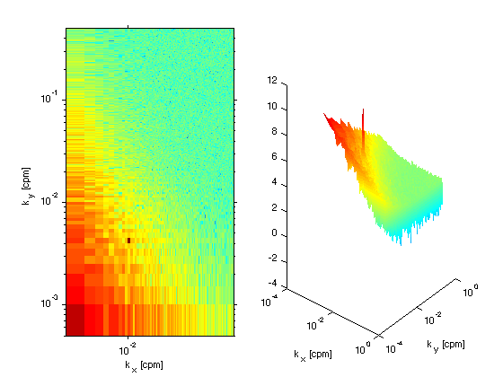
Do the 2-D spectral estimate...
XY = fft(fft(w')');
k_x = (0:M-1)/dx/M;
k_y = (0:N-1)/dx/N;

GXY = (1/M/dx)*(1/N/dy)*XY(2:N/2,2:M/2).* conj(XY(2:N/2,2:M/2));
k_y = k_y(2:N/2);
k_x = k_x(2:M/2);
Note how the spectrum has large amlitude at low wavenumbers, and then hits a noise floor at high wavenumbers.
figure(15);clf
subplot(1,2,1);

pcolor(k_x,k_y,log10(real(GXY)));shading flat;
set(gca,'xscale','log','yscale','log')
xlabel('k_x [cpm]');
ylabel('k_y [cpm]');

subplot(1,2,2);

surface(k_x,k_y,log10(real(GXY)));shading interp;
set(gca,'xscale','log','yscale','log')
xlabel('k_x [cpm]');
ylabel('k_y [cpm]');
view(40,20);