Making a Power Spectrum

Getting started
Compute a raw fft
Computing the frequencies
Plotting the FFT amplitudes.
Normalizing the spectrum

Getting started

load SynthSig;

Compute a raw fft

Make this the white noise process. Note that X is a complex quantity. Also note that X has the same size as x. Therefore, no information is lost.

We want dimensional spectra, so we multiply the FFT by dt.

dt = median(diff(sig.t));

size(sig.x_r)
X = dt*fft(sig.x+sig.x_peak*10);
X(1:4)
size(X)

ans =

           1        2001


ans =

   1.0e+02 *

   7.8893             0.4028 + 2.4841i   0.1274 + 1.1476i  -0.0198 + 0.2030i


ans =

           1        2001

we can invert to recover the original signal

temp = ifft(X);
temp(1:4)
sig.x_r(1:4)

ans =

    1.2890    1.0057    0.4859    0.1502


ans =

    0.1201    0.2291    0.1932    0.1802

Computing the frequencies

Matlab normalizes everything so the time between data points is unity. These frequencies are (k-1)/N, 1<=k<=N. In order to get dimensional frequencies, we need

dt = median(diff(sig.t));
N = length(sig.x);
f = (0:N-1)/N/dt;

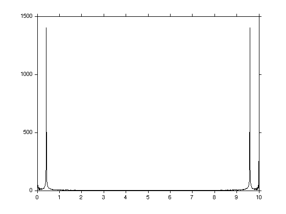
Plotting the FFT amplitudes.

Note that the high frequencies and the low frequencies look suspiciously similar.

figure(1);clf
plot(f,abs(X))

It can easily be shown that if x is real then X(1+i)=X(N+1-i), i>1.

X(1+6)
X(N+1-6)

ans =

   6.5510 +46.8497i


ans =

   6.5510 -46.8497i

since half the spectrum is not used, it is usual to drop it from consideration.

Px=X(1:((N-1)/2)+1).*conj(X(1:((N-1)/2)+1));
f=f(1:((N-1)/2)+1);

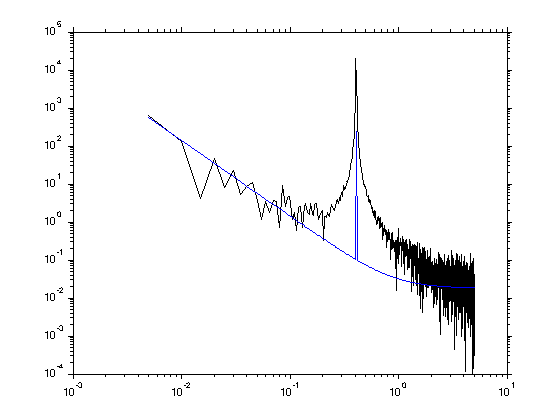
Normalizing the spectrum

At this point we still have a dimensionless spectrum. We want sum(Px*df)=var(x) so the appropriate normalization turns out to be:

Px = Px*2/N/dt;

loglog(f,Px,th.f,th.Px);