Problems w/ power spectra?

Contents

Getting started

load SynthSig;

Aliasing

Here we need to generate another peak.

om_peak= 4.4*2*pi;
ph = rand(1,1)*2*pi;

sig.x_peak2 = 2*10.*cos(om_peak*sig.t+ph)/10;

[p,f]=rawPowerSpec(sig.x_peak2+sig.x_peak+sig.x_w,dt);

% Now, suppose that we can only sample at 0.25 Hz (i.e. 1/4 of the time)
xx = sig.x_peak2+sig.x_peak+sig.x_w;

x=xx(1:4:end);
t = sig.t(1:4:end);
[pn,fn]=rawPowerSpec(x,median(diff(t)));

jmkfigure(100,2,0.6);clf
subplot(2,1,1);
plot(x(1:100));
hold on;
plot(1:4:100,x(1:4:100),'b.','markersi',10);
xlabel('t [s]');
ylabel('x [m]');


subplot(2,1,2);

loglog(f,p,fn,pn)
axis tight;
yl = get(gca,'ylim');
xlabel('f [Hz]');
ylabel('\phi_x [m^2 s^{-1}]');
axis tight
print -dpng -r250 doc/Aliasing

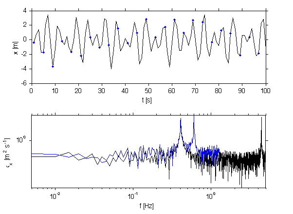
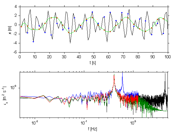
here we see the result of aliasing, where the peak has wrapped around to a harmonic in the resolved spectrum. To stop this we should smooth the new signal first:

[b,a]=butter(2,0.3);
x = filtfilt(b,a,xx);
subplot(2,1,1);
plot(1:4:100,x(1:4:100),'r.','markersize',10)
plot(x(1:100),'g')
xlabel('t [s]');
ylabel('x [m]');

[pnp,fnp]=rawPowerSpec(x,median(diff(sig.t)));
x = x(1:4:end);
t = sig.t(1:4:end);
[pnn,fnn]=rawPowerSpec(x,median(diff(t)));
subplot(2,1,2);
loglog(f,p,fn,pn,fnp,pnp,fnn,pnn)
set(gca,'ylim',yl);
xlabel('f [Hz]');
ylabel('\phi_x [m^2 s^{-1}]');
axis tight
print -dpng -r250 doc/AliasingFixed

Finite record length

The last foible is finite record length. The difference between frequency bins is df = 1/T where T is the length of the record. Shorter records, the longer df.

To see the effect make a second peak very close to the first, but far enough apart that they can be distinguished in the full time-series.

om = th.f*2*pi;
om_peak = find(om>0.4*2*pi);
f0=om(om_peak(1))/2/pi;

om_peak=om(om_peak(1)+3); % chose a peak 4 bins higher.
ff = om_peak/2/pi;
1./abs(ff-f0)

ph = rand(1,1)*2*pi;

sig.x_peak2 = A_peak.*cos(om_peak*sig.t+ph)/10;

x = sig.x_peak2+sig.x_peak+sig.x_w;

jmkfigure(3,2,0.7);clf
subplot(3,1,1);
plot(x);
hold on;
plot(x(1:1500),'b');
plot(x(1:1000),'r');
ylabel('x [m]');

subplot(3,1,[2 3]);
sty = {'k-','b-','r-'};
N = length(x);
for i=1:3;
  [p,f]=rawPowerSpec(x(1:N-0.35*N*(i-1)),dt);
  loglog(f,p,sty{i});
  hold on;
  h(i)=loglog(f,p,'o','markersi',6,'col',sty{i}(1));
  set(gca,'xlim',[1.1*10^(-0.5) 1.7*10^(-0.5)]);
  df(i)=median(diff(f));
  nn(i) = length(x(1:N-0.25*N*(i-1)));
  str{i}=sprintf('N=%d; \\Delta f=%1.2e [Hz]',nn(i),df(i));
end;
xlabel('f [Hz]');
ylabel('\phi_x [m^2 Hz^{-1}]');

legend(h(1:3),str{1:3})
title(sprintf('Peaks separated by \\Delta f=%1.2e',abs(ff-f0)));
print -dpng -r400 doc/FiniteRecord.jpg

ans =

   66.6667

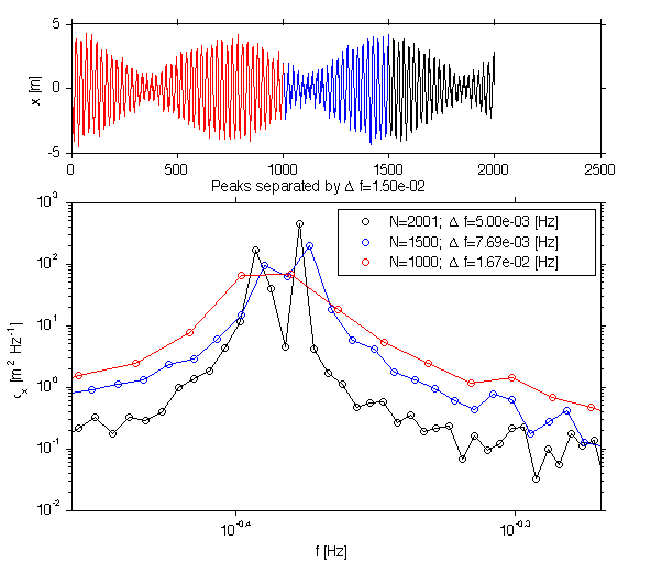
Here it is clear that fewer data points means poorer peak resolution. Once df rises above the peak separation they merge.

A trick to get better frequency resolution is to zero-pad the data. However, in this case, even if we do this, we do not improve resolution between the peaks, just the centering of the peaks.

jmkfigure(4,2,0.6);clf
sty = {'k-','b-','r-'};
N = length(x);
for i=1:3;
  subplot3(1,3,i,'xscale','log','yscale','log');
  [p,f]=rawPowerSpec(x(1:N-0.35*N*(i-1)),dt);
  loglog(f,p,sty{i});

  xx = x(1:N-0.35*N*(i-1));
  xxx = zeros(1,floor(5*N));
  xxx(1:length(xx)) =xx;

  [pp,ff]=rawPowerSpec(xxx,dt);
  h(i)=loglog(ff,pp,sty{i});
  hold on;
  h(i)=loglog(f,p,sty{i});
  hold on;
  %  h(i)=loglog(f,p,'o','markersi',6,'col',sty{i}(1));
  set(gca,'xlim',[1.1*10^(-0.5) 1.7*10^(-0.5)]);
  df(i)=median(diff(f));
  nn(i) = length(x(1:N-0.25*N*(i-1)));
  str{i}=sprintf('N=%d',nn(i));
  if i==1
    ylabel('\phi_x [m^2 Hz^{-1}]');
  end;
end;

%legend(h(1:3),str{1:3})
title('Zero-padded data');
xlabel('f [Hz]');
print -dpng -r400 doc/ZeroPad.jpg

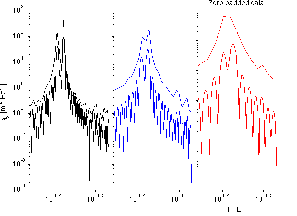
Note in this example how the poorly-resolved peaks (blue) have better peak localization than if we don't zero pad. However, this doesn't help separate peaks that aren't resolved in the unpadded timeseries.

Spectral Leakage:

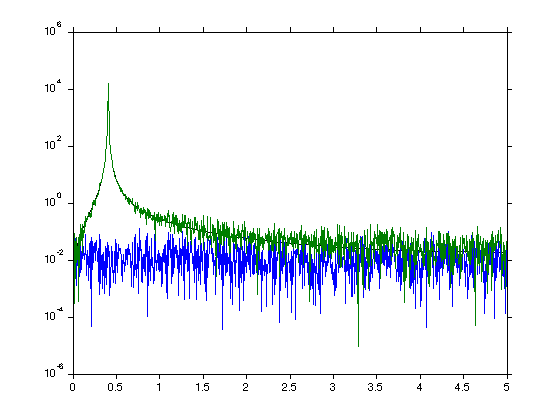
Compute a raw fft of a strong peak with white noise. Note that we have put the steps from the previous tutorial into a function.

dt = median(diff(sig.t))
[p,f]=rawPowerSpec(sig.x_peak*10,dt);

[p_w,f]=rawPowerSpec(sig.x_w,dt);
[p_p,f]=rawPowerSpec(sig.x_peak*10+sig.x_w,dt);

figure(1);clf
semilogy(f,p,f,p_w,f,p_p);

dt =

    0.1000

Next

Next we consider ways to reduce smearing of peaks in the spectra and ways to improve the signal-to-noise of spectral extimates.

Published with MATLAB® 7.7