FFT first tutorial..

Introduction
Synthesized data
Theoretical power spectra

Introduction

This tutorial deals with Fourier analysis and its use in interpreting data. The reader is assumed to be familiar with Fourier transforms, but not necessarily with their use in data characterization.

Synthesized data

Here we create a synthetic data set consisting of a "red" signal, an isolated peak, and "white" noise.

First, the time axis is determined. Note this could be a spatial axis as well. This data has a sampling frequency of dt. We could use dt=1, but this lends considerable confusion later when determining the amplitude of the spectrum.

dt = 0.1; % seconds
t = (0:2000)*0.1;

We will have data with frequencies of 1/dt/2 to 1/1000; Note that we keep track of units as factors of 2*pi can easily be lost when dealing with the frequency domain.

dom = 1/200;
om = dom:dom:1/dt/2; % this is cycles/s=Hz.
om = 2*pi*om;  % this is rad/s.

set the relative amplitudes:

A_w = 0.3;
A_r = 1;
A_peak = 22;
om_peak = find(om>0.4*2*pi);
% make sure it is not dead on a peak
om_peak=om(om_peak(1))+0.3*median(diff(om));

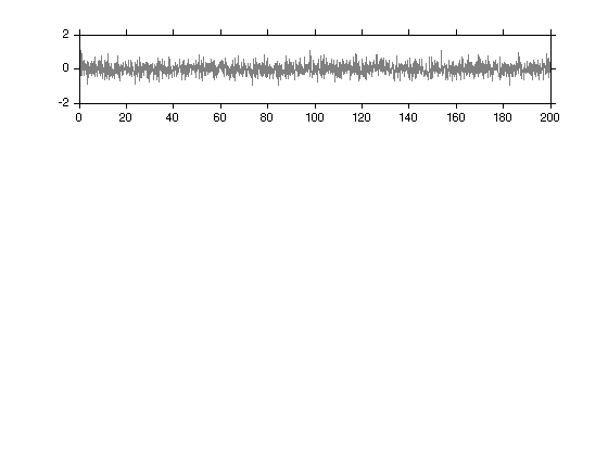
White noise is a Gaussian process...

x_w = A_w*randn(1,length(t));

figure(1);
subplot(4,1,1);
plot(t,x_w,'col',[1 1 1]*0.5);

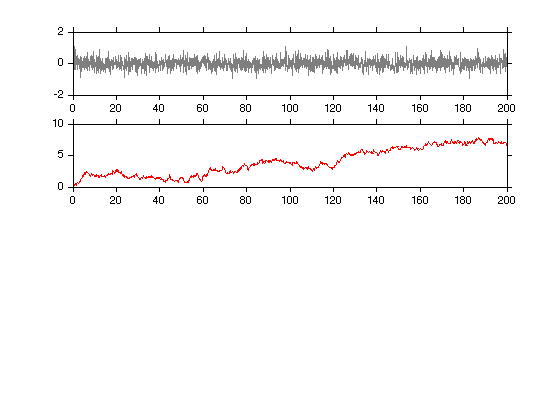
A Red signal is the integral of a Gaussian process.

%A   = repmat(A_r*(1+0.9*randn(length(om),1)).*om'.^(-1),1,length(t));
%ph = repmat(rand(length(om),1)*2*pi,1,length(t));

%x_r = sum(A.*cos(om'*t+ph))*sqrt(dom);
x_r = cumsum(randn(1,length(t)))*median(diff(t));

subplot(4,1,2);
plot(t,x_r,'r');

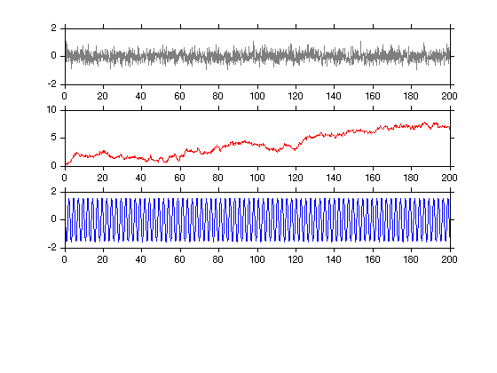
A peak

ph = rand(1,1)*2*pi;

x_peak = A_peak.*cos(om_peak*t+ph)*sqrt(dom);

subplot(4,1,3);
plot(t,x_peak,'b');

Combine...

x=x_peak+x_r+x_w;

subplot(4,1,4);
plot(t,x);
set(datachildren(gcf),'ylim',[-1 1]*10);
ylabel('x [m]');

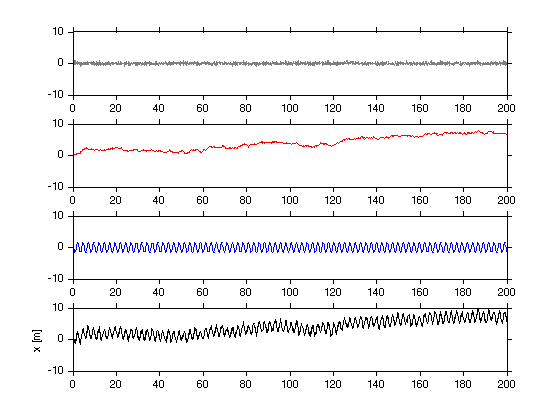
Theoretical power spectra

The three wave forms plotted above have known power spectra.

f = om/2/pi;
df = median(diff(f)); % it is usual to plot spectra in terms of cycles/s.
P_w = om*0+var(x_w)/max(f);

P_r = f.^(-2);
P_r = P_r./sum(P_r*df)*var(x_r);

P_peak = om*0;
in = find(om>=om_peak);in =in(1)
P_peak(in) = 1*var(x_peak)/df;
% rename so we don't overwrite by accident.
th.f=f;
th.P_r=P_r;
th.P_w=P_w;
th.P_peak=P_peak;
th.Px = th.P_r+th.P_w+th.P_peak;
%
sig.t =t;
sig.x_w = x_w;
sig.x_r = x_r;
sig.x_peak = x_peak;
sig.x = x;

jmkfigure(2,2,0.4);clf
loglog(th.f,th.P_w,'col',[1 1 1]*0.5);
hold on;
loglog(th.f,th.P_r,'r');
loglog(th.f,th.P_peak,'bx','markersi',10);
loglog(th.f,th.Px,'k');
xlabel('f [Hz]');
ylabel('P_x [m^2 Hz^{-1}]');
legend('x_w','x_r','x_{peak}','Sum');
title('Theoretical spectrum of synthetic signals');

in =

    82

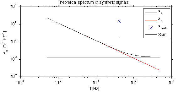
The plot shown above is the ideal we are striving towards. With infinite samples of the processes the power spectra would look like what is given above.

save SynthSig sig th

if 0
  warning off;
  opt.outputDir='/Users/jklymak/Sites/Phy580/html';
  publish('FftSynthesizeData',opt);
end;

FFT first tutorial..

Contents

Introduction

Synthesized data

Theoretical power spectra