Improving confidence in power spectra
Contents
Getting started
load SynthSig;
Intro
In the previous two tutorials we saw that there are some shortcomings to simply taking the raw powerspectra. First, if there is a large peak in the data it can leak energy to surrounding frequencies. Second, it is typically desirable to distinguish if a peak is significant. This typically requires some sort of averaging technique.
Reducing leakage.
The favoured method for reducing leakage is to window the data before performing the fft.
x = sig.x_peak;
N = length(x);
W = hanning(N)';
W = W./sqrt(mean(abs(W).^2));
y = x.*W;
dt=median(diff(sig.t));
[px,f]=rawPowerSpec(x,dt);


figure(2);
clf
subplot(2,1,1);
plot(sig.t,x);
hold on;
ylabel('x [m]');
xlabel('t [s]');

subplot(2,1,2);
loglog(f,px);
hold on;
set(gca,'ylim',[1e-6 1e3]);
xlabel('F [Hz]');
ylabel('\phi_x [m^2 Hz^{-1}]');

print -dpng -r250 doc/NoWindow


subplot(2,1,1);
plot(sig.t,y,'b');

[py,f]=rawPowerSpec(y,dt);
subplot(2,1,2);
loglog(f,py,'b');
print -dpng -r250 doc/Window
set(gca,'xlim',[0.2 0.8]);
print -dpng -r250 doc/WindowZoom
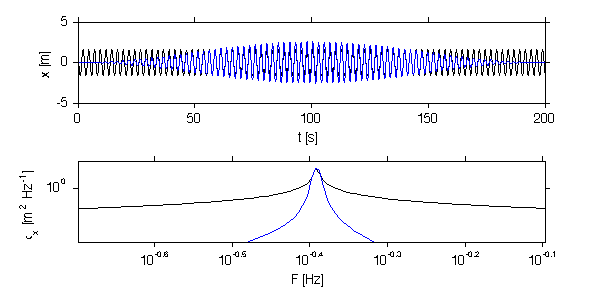
Here we see how applying the window has tightened the spectrum. Note however, that the peak has been spread a little bit into adjoining bins. Lets try on a braodband spectrum. Note that here we have to make the peak very prominent to make the effect important. However, also notice that the rest of the spectrum is not unduly disturbed.
figure(12);clf

x = sig.x+30*sig.x_peak;
W = hanning(N)';
W = N*W./sum(W);
y = x.*W;
clf
subplot(3,1,1);
plot(sig.t,x,sig.t,y);
dt=median(diff(sig.t));


[px,f]=rawPowerSpec(x,dt);
[py,f]=rawPowerSpec(y,dt);
subplot(3,1,2);
loglog(f,px,f,py);
set(gca,'ylim',[1e-6 1e6]);
xlabel('F [Hz]');
ylabel('\phi_x [m^2 Hz^{-1}]');
subplot(3,1,3);
loglog(f,px,f,py);
set(gca,'ylim',[1e-2 1e6]);
xlabel('F [Hz]');
ylabel('\phi_x [m^2 Hz^{-1}]');
set(gca,'xlim',[1e-1 10e-1]);
print -dpng -r250 doc/TaperingAgain

The Periodigram
The next procedure that is often carried out is to average the data somewhat. This can reveal shapes to the spectra that are not readily apparent in their rougher form.
The most common technique is the periodigram. This is accomplished by reshaping the data into blocks nfft long, windowing the data, and then taking the fft on each block. The resulting spectra are averaged. Because the windowing removes data at the edges, it is usual to overlap the windows by at least 50%. The overlapping logic requires a bit of care,
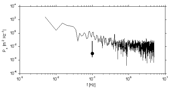
x = sig.x_r+sig.x_w+sig.x_peak/10;
[px0,f0]=rawPowerSpec(detrend(x,0),dt);


jmkfigure(11,2,0.4);clf
[p,f,dof0,conf0]=periodogramPowerSpec(x,dt,length(x));
loglog(f,p);
line([0.1 0.1],conf0/1000,'linesty','-','linewi',2)
hold on;plot([0.1],1/1000,'o','markerfacecol','k','markersi',10)

xlabel('f [Hz]');
ylabel('P_x [m^2 Hz^{-1}]');
if dop
  docprint('ConfInterval','FftTechniques.m');
end;
N =

        2001


nind =

     1
Spectral Smoothing...
First, lets do the most obvious thing and smooth the spectra in frequency space...
psmooth = conv2(p,ones(1,10)/10,'same')
loglog(f,psmooth,'b');
% set(gca,'xlim',[0.06 1])
line([0.1 0.1],conf0/1000,'linesty','-','linewi',2)

if dop
  docprint('FreqSmooth','FftTechniques.m');
end;
psmooth =

  Columns 1 through 8

   32.1506   32.5134   32.5201   32.6132   32.6522    7.5511    7.3925    4.1905

  Columns 9 through 16

    2.7564    1.6744    0.9328    0.7766    0.8286    0.7602    0.8528    0.9494

  Columns 17 through 24

    0.8577    0.8117    0.8074    0.8021    0.6978    0.5343    0.5057    0.4851

  Columns 25 through 32

    0.3695    0.2425    0.2192    0.1943    0.2269    0.2426    0.1954    0.1699

  Columns 33 through 40

    0.1404    0.1463    0.1506    0.1726    0.1854    0.1949    0.1540    0.1317

  Columns 41 through 48

    0.1470    0.1479    0.1530    0.1461    0.1284    0.0928    0.0751    0.0643

  Columns 49 through 56

    0.0647    0.0594    0.0561    0.0566    0.0568    0.0560    0.0639    0.0827

  Columns 57 through 64

    0.0995    0.1122    0.1161    0.1227    0.1289    0.1119    0.1099    0.1094

  Columns 65 through 72

    0.1001    0.0831    0.0666    0.0534    0.0568    0.0501    0.0291    0.0299

  Columns 73 through 80

    0.0329    0.0340    0.0373    0.1031    0.1625    0.1646    0.1561    0.1641

  Columns 81 through 88

    0.1720    0.1694    0.1687    0.1681    0.1684    0.1048    0.0443    0.0394

  Columns 89 through 96

    0.0415    0.0369    0.0328    0.0379    0.0376    0.0360    0.0312    0.0298

  Columns 97 through 104

    0.0349    0.0350    0.0318    0.0291    0.0291    0.0257    0.0269    0.0351

  Columns 105 through 112

    0.0389    0.0415    0.0421    0.0421    0.0445    0.0431    0.0404    0.0405

  Columns 113 through 120

    0.0339    0.0286    0.0326    0.0354    0.0318    0.0311    0.0302    0.0339

  Columns 121 through 128

    0.0328    0.0335    0.0386    0.0462    0.0447    0.0358    0.0340    0.0351

  Columns 129 through 136

    0.0336    0.0301    0.0318    0.0352    0.0314    0.0203    0.0148    0.0178

  Columns 137 through 144

    0.0287    0.0382    0.0438    0.0459    0.0440    0.0381    0.0376    0.0386

  Columns 145 through 152

    0.0377    0.0347    0.0298    0.0362    0.0324    0.0349    0.0385    0.0387

  Columns 153 through 160

    0.0394    0.0391    0.0394    0.0398    0.0331    0.0169    0.0154    0.0133

  Columns 161 through 168

    0.0119    0.0120    0.0106    0.0139    0.0135    0.0176    0.0214    0.0244

  Columns 169 through 176

    0.0248    0.0213    0.0224    0.0260    0.0266    0.0245    0.0272    0.0226

  Columns 177 through 184

    0.0193    0.0156    0.0145    0.0146    0.0113    0.0094    0.0130    0.0160

  Columns 185 through 192

    0.0234    0.0283    0.0296    0.0313    0.0349    0.0394    0.0404    0.0400

  Columns 193 through 200

    0.0447    0.0417    0.0343    0.0326    0.0315    0.0307    0.0283    0.0249

  Columns 201 through 208

    0.0253    0.0282    0.0247    0.0261    0.0264    0.0268    0.0325    0.0409

  Columns 209 through 216

    0.0413    0.0405    0.0407    0.0379    0.0324    0.0304    0.0304    0.0273

  Columns 217 through 224

    0.0226    0.0138    0.0137    0.0163    0.0169    0.0151    0.0155    0.0183

  Columns 225 through 232

    0.0167    0.0179    0.0180    0.0192    0.0181    0.0168    0.0156    0.0193

  Columns 233 through 240

    0.0230    0.0213    0.0206    0.0191    0.0176    0.0171    0.0175    0.0163

  Columns 241 through 248

    0.0183    0.0175    0.0164    0.0151    0.0161    0.0185    0.0245    0.0347

  Columns 249 through 256

    0.0349    0.0360    0.0332    0.0315    0.0296    0.0293    0.0314    0.0320

  Columns 257 through 264

    0.0301    0.0275    0.0295    0.0291    0.0290    0.0295    0.0315    0.0330

  Columns 265 through 272

    0.0346    0.0378    0.0356    0.0275    0.0247    0.0240    0.0258    0.0250

  Columns 273 through 280

    0.0222    0.0205    0.0171    0.0114    0.0092    0.0104    0.0130    0.0153

  Columns 281 through 288

    0.0155    0.0155    0.0155    0.0178    0.0160    0.0170    0.0193    0.0191

  Columns 289 through 296

    0.0163    0.0168    0.0166    0.0162    0.0168    0.0163    0.0252    0.0340

  Columns 297 through 304

    0.0353    0.0361    0.0363    0.0335    0.0316    0.0315    0.0311    0.0313

  Columns 305 through 312

    0.0293    0.0209    0.0181    0.0177    0.0184    0.0186    0.0192    0.0229

  Columns 313 through 320

    0.0243    0.0240    0.0185    0.0179    0.0187    0.0195    0.0214    0.0233

  Columns 321 through 328

    0.0241    0.0216    0.0214    0.0197    0.0211    0.0221    0.0213    0.0207

  Columns 329 through 336

    0.0202    0.0190    0.0178    0.0191    0.0190    0.0204    0.0220    0.0236

  Columns 337 through 344

    0.0233    0.0250    0.0262    0.0260    0.0278    0.0306    0.0381    0.0402

  Columns 345 through 352

    0.0379    0.0341    0.0348    0.0338    0.0313    0.0306    0.0299    0.0246

  Columns 353 through 360

    0.0164    0.0157    0.0162    0.0172    0.0165    0.0140    0.0137    0.0154

  Columns 361 through 368

    0.0153    0.0147    0.0147    0.0154    0.0196    0.0224    0.0242    0.0256

  Columns 369 through 376

    0.0260    0.0256    0.0291    0.0325    0.0339    0.0337    0.0313    0.0289

  Columns 377 through 384

    0.0275    0.0271    0.0286    0.0339    0.0376    0.0352    0.0328    0.0287

  Columns 385 through 392

    0.0247    0.0237    0.0234    0.0224    0.0219    0.0196    0.0131    0.0137

  Columns 393 through 400

    0.0141    0.0142    0.0142    0.0138    0.0131    0.0130    0.0112    0.0105

  Columns 401 through 408

    0.0096    0.0109    0.0136    0.0155    0.0165    0.0171    0.0211    0.0221

  Columns 409 through 416

    0.0216    0.0180    0.0174    0.0145    0.0113    0.0097    0.0092    0.0091

  Columns 417 through 424

    0.0057    0.0046    0.0050    0.0110    0.0154    0.0153    0.0172    0.0193

  Columns 425 through 432

    0.0192    0.0192    0.0195    0.0195    0.0203    0.0157    0.0130    0.0142

  Columns 433 through 440

    0.0122    0.0108    0.0108    0.0108    0.0104    0.0104    0.0095    0.0080

  Columns 441 through 448

    0.0058    0.0051    0.0055    0.0048    0.0058    0.0083    0.0091    0.0103

  Columns 449 through 456

    0.0117    0.0120    0.0153    0.0172    0.0181    0.0188    0.0177    0.0164

  Columns 457 through 464

    0.0170    0.0156    0.0170    0.0177    0.0174    0.0179    0.0174    0.0165

  Columns 465 through 472

    0.0163    0.0154    0.0177    0.0266    0.0308    0.0349    0.0323    0.0310

  Columns 473 through 480

    0.0333    0.0335    0.0350    0.0359    0.0323    0.0239    0.0177    0.0151

  Columns 481 through 488

    0.0190    0.0240    0.0272    0.0279    0.0266    0.0247    0.0251    0.0269

  Columns 489 through 496

    0.0257    0.0240    0.0208    0.0147    0.0084    0.0075    0.0076    0.0084

  Columns 497 through 504

    0.0083    0.0081    0.0099    0.0103    0.0093    0.0096    0.0100    0.0136

  Columns 505 through 512

    0.0180    0.0198    0.0200    0.0183    0.0183    0.0224    0.0249    0.0250

  Columns 513 through 520

    0.0268    0.0254    0.0207    0.0182    0.0175    0.0169    0.0150    0.0099

  Columns 521 through 528

    0.0127    0.0179    0.0172    0.0162    0.0161    0.0175    0.0221    0.0251

  Columns 529 through 536

    0.0255    0.0314    0.0330    0.0280    0.0279    0.0271    0.0269    0.0256

  Columns 537 through 544

    0.0212    0.0193    0.0193    0.0159    0.0121    0.0121    0.0117    0.0127

  Columns 545 through 552

    0.0131    0.0131    0.0127    0.0123    0.0119    0.0101    0.0100    0.0111

  Columns 553 through 560

    0.0108    0.0093    0.0100    0.0139    0.0157    0.0154    0.0154    0.0151

  Columns 561 through 568

    0.0139    0.0162    0.0180    0.0182    0.0169    0.0139    0.0123    0.0138

  Columns 569 through 576

    0.0189    0.0229    0.0235    0.0225    0.0251    0.0300    0.0317    0.0312

  Columns 577 through 584

    0.0310    0.0300    0.0258    0.0216    0.0190    0.0157    0.0107    0.0066

  Columns 585 through 592

    0.0066    0.0102    0.0129    0.0122    0.0114    0.0116    0.0125    0.0144

  Columns 593 through 600

    0.0171    0.0168    0.0151    0.0112    0.0080    0.0080    0.0088    0.0104

  Columns 601 through 608

    0.0097    0.0079    0.0060    0.0141    0.0303    0.0408    0.0436    0.0458

  Columns 609 through 616

    0.0511    0.0529    0.0562    0.0589    0.0589    0.0512    0.0367    0.0270

  Columns 617 through 624

    0.0251    0.0232    0.0173    0.0142    0.0115    0.0113    0.0112    0.0109

  Columns 625 through 632

    0.0131    0.0126    0.0123    0.0122    0.0125    0.0123    0.0115    0.0089

  Columns 633 through 640

    0.0096    0.0109    0.0070    0.0076    0.0079    0.0075    0.0067    0.0076

  Columns 641 through 648

    0.0125    0.0160    0.0149    0.0125    0.0128    0.0128    0.0168    0.0200

  Columns 649 through 656

    0.0215    0.0230    0.0217    0.0197    0.0208    0.0215    0.0216    0.0217

  Columns 657 through 664

    0.0224    0.0196    0.0211    0.0190    0.0161    0.0147    0.0150    0.0142

  Columns 665 through 672

    0.0140    0.0129    0.0083    0.0082    0.0057    0.0052    0.0045    0.0049

  Columns 673 through 680

    0.0043    0.0097    0.0115    0.0116    0.0117    0.0117    0.0111    0.0111

  Columns 681 through 688

    0.0166    0.0201    0.0199    0.0152    0.0135    0.0146    0.0183    0.0215

  Columns 689 through 696

    0.0252    0.0271    0.0266    0.0234    0.0229    0.0242    0.0272    0.0283

  Columns 697 through 704

    0.0292    0.0299    0.0270    0.0249    0.0206    0.0229    0.0293    0.0320

  Columns 705 through 712

    0.0293    0.0295    0.0266    0.0233    0.0226    0.0239    0.0249    0.0264

  Columns 713 through 720

    0.0250    0.0211    0.0214    0.0218    0.0213    0.0218    0.0227    0.0245

  Columns 721 through 728

    0.0281    0.0264    0.0213    0.0213    0.0206    0.0183    0.0164    0.0175

  Columns 729 through 736

    0.0208    0.0228    0.0206    0.0184    0.0201    0.0224    0.0229    0.0222

  Columns 737 through 744

    0.0221    0.0197    0.0163    0.0109    0.0085    0.0086    0.0069    0.0043

  Columns 745 through 752

    0.0046    0.0056    0.0057    0.0057    0.0065    0.0101    0.0095    0.0087

  Columns 753 through 760

    0.0092    0.0099    0.0139    0.0188    0.0200    0.0202    0.0198    0.0178

  Columns 761 through 768

    0.0188    0.0199    0.0200    0.0190    0.0166    0.0116    0.0108    0.0115

  Columns 769 through 776

    0.0117    0.0103    0.0097    0.0095    0.0113    0.0126    0.0113    0.0117

  Columns 777 through 784

    0.0113    0.0110    0.0103    0.0123    0.0133    0.0122    0.0114    0.0102

  Columns 785 through 792

    0.0160    0.0188    0.0215    0.0241    0.0236    0.0214    0.0202    0.0213

  Columns 793 through 800

    0.0203    0.0201    0.0137    0.0098    0.0075    0.0062    0.0067    0.0075

  Columns 801 through 808

    0.0080    0.0072    0.0078    0.0100    0.0109    0.0113    0.0107    0.0098

  Columns 809 through 816

    0.0094    0.0110    0.0198    0.0260    0.0263    0.0256    0.0272    0.0280

  Columns 817 through 824

    0.0280    0.0286    0.0300    0.0278    0.0254    0.0267    0.0269    0.0266

  Columns 825 through 832

    0.0308    0.0333    0.0345    0.0356    0.0359    0.0370    0.0300    0.0228

  Columns 833 through 840

    0.0229    0.0222    0.0151    0.0114    0.0108    0.0117    0.0116    0.0110

  Columns 841 through 848

    0.0109    0.0120    0.0125    0.0134    0.0142    0.0142    0.0143    0.0130

  Columns 849 through 856

    0.0149    0.0163    0.0165    0.0176    0.0204    0.0227    0.0254    0.0259

  Columns 857 through 864

    0.0253    0.0232    0.0206    0.0226    0.0226    0.0223    0.0177    0.0138

  Columns 865 through 872

    0.0115    0.0143    0.0160    0.0169    0.0155    0.0135    0.0163    0.0157

  Columns 873 through 880

    0.0155    0.0188    0.0187    0.0156    0.0140    0.0142    0.0142    0.0123

  Columns 881 through 888

    0.0094    0.0077    0.0084    0.0054    0.0058    0.0064    0.0062    0.0061

  Columns 889 through 896

    0.0074    0.0075    0.0077    0.0082    0.0088    0.0141    0.0203    0.0259

  Columns 897 through 904

    0.0293    0.0298    0.0288    0.0287    0.0290    0.0290    0.0277    0.0220

  Columns 905 through 912

    0.0142    0.0077    0.0046    0.0035    0.0046    0.0052    0.0049    0.0046

  Columns 913 through 920

    0.0051    0.0097    0.0127    0.0148    0.0150    0.0151    0.0139    0.0156

  Columns 921 through 928

    0.0163    0.0172    0.0171    0.0128    0.0124    0.0164    0.0232    0.0274

  Columns 929 through 936

    0.0321    0.0321    0.0312    0.0325    0.0366    0.0377    0.0376    0.0342

  Columns 937 through 944

    0.0280    0.0235    0.0210    0.0222    0.0232    0.0209    0.0172    0.0160

  Columns 945 through 952

    0.0137    0.0108    0.0097    0.0103    0.0086    0.0072    0.0095    0.0119

  Columns 953 through 960

    0.0129    0.0148    0.0166    0.0181    0.0183    0.0194    0.0210    0.0201

  Columns 961 through 968

    0.0169    0.0146    0.0149    0.0168    0.0174    0.0168    0.0181    0.0182

  Columns 969 through 976

    0.0168    0.0161    0.0174    0.0184    0.0167    0.0137    0.0117    0.0109

  Columns 977 through 984

    0.0096    0.0081    0.0068    0.0070    0.0067    0.0064    0.0078    0.0070

  Columns 985 through 992

    0.0064    0.0062    0.0073    0.0071    0.0077    0.0073    0.0067    0.0060

  Columns 993 through 1000

    0.0043    0.0065    0.0140    0.0138    0.0122    0.0121    0.0115    0.0111
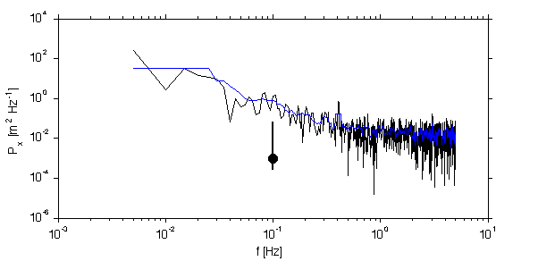
logarithmic smoothing...
loglog(f,logsmooth(p),'r');
if dop
  docprint('LogSmooth','FftTechniques.m');
end;

Periodigrams with incremental smoothing and confidence intervals...
Periodigram...
jmkfigure(12,2,0.8);
clf
subplot(3,1,1);
loglog(f0,px0);
hold on;

% Theoretical power spectra
% The three wave forms plotted above have known power spectra.
f = f0;
df = median(diff(f)); % it is usual to plot spectra in terms of cycles/s.
P_w = f*0+var(sig.x_w)/max(f);

P_r = f.^(-2);
P_r = P_r./sum(P_r*df)*var(sig.x_r);

P_peak = f*0;

%in = find(om==om_peak);
%P_peak(in) = 1*var(sig.x_peak)/df/10;
% rename so we don't overwrite by accident.
th.f=f;
th.P_r=P_r;
th.P_w=P_w;
th.P_peak=P_peak;
th.Px = th.P_r+th.P_w+th.P_peak;
%

loglog(th.f,th.P_w,'col',[1 1 1]*0.5);
hold on;
loglog(th.f,th.P_r,'r');
loglog(th.f,th.P_peak,'bx','markersi',10);
loglog(th.f,th.Px,'k');
xlabel('f [Hz]');
ylabel('P_x [m^2 Hz^{-1}]');
title('Theoretical spectrum of synthetic signals');

set(gca,'ylim',[1e-2 5e2]);

nfft_in = 512/2;
N = length(x)
nfft=min([nfft_in N]);
repeats=round(2*N/nfft)

starts = floor(linspace(1,N-nfft,repeats))

X = [1:nfft]'*ones(1,repeats);
X = ceil(X+ones(nfft,1)*(starts-1));
t = sig.t;
x0 = x;t0=t;

x = x(floor(X));
t = t(floor(X));

% must remove the trend from each block
x = detrend(x,0);

W = hanning(nfft)';
W = sqrt(nfft)*W./norm(W);
W = W./sqrt(mean(W.^2));
x = x.*repmat(W',1,size(x,2));

subplot(3,1,2);
plot(t,x);
hold on;
plot(t0,x0+3);
xlabel('t [s]');
ylabel('x [m]');

Px = dt*fft(x);
dt = median(diff(sig.t));
N = nfft;
if mod(N,2)==1
  nn = nfft;
else
  nn=nfft-1;
end;

f = (0:nfft-1)/nfft/dt;
f = f(2:(nn/2));
Px = Px(2:(nn/2),:);
Px =Px.*conj(Px)*2/dt/N;

subplot(3,1,3);
loglog(f,Px)
hold on;
loglog(f,nanmean(Px'),'linewi',2)
loglog(th.f,th.Px,'linewi',1)
set(gca,'ylim',[1e-2 1e2],'xlim',[1e-3 10]);
xlabel('f [Hz]');
ylabel('P_x [m^2 Hz^{-1}]');
print -dpng -r200 doc/PeriodigramTech
N =

        2001


repeats =

    16


starts =

  Columns 1 through 7

           1         117         233         349         466         582         698

  Columns 8 through 14

         814         931        1047        1163        1279        1396        1512

  Columns 15 through 16

        1628        1745
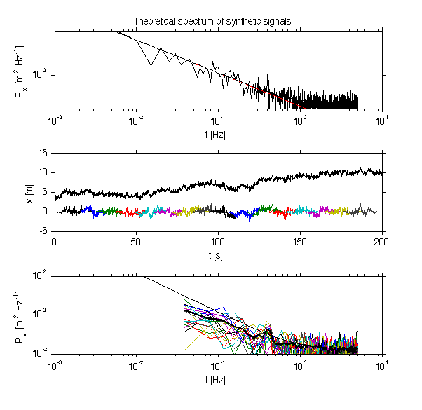
We can package th is procedure up into a periodigram m-file
Here we compare the results from 4 different fft lengths. The degrees of freedom and confidence intervals (in logarithmic space) are given. Note the peak only becomes statistically significant for nfft=512.
Also note the tradeoffs. The peak is less well resolved for shorter nfft. And less of the lower frequencies are resilved.
The other advantage, though, is a smoother resolution of the spectra at other frequencies. The take-home lesson is that a variety of spectral methods should be tried if the goal is data interpretation.
jmkfigure(3,2,0.5);clf
nfft = fliplr(256*[1 2 4 (length(x))/256]);
x = 2*sig.x_r+sig.x_w+sig.x_peak/10;
col ={'r','g','b','m'};
for i=1:length(nfft);
  [p,f,dof(i),conf(i,:)]=periodogramPowerSpec(x,dt,nfft(i));
 % [pp,ff]=pwelch(x,hanning(nfft(i)),nfft(i)/2,nfft(i),1/dt);
  loglog(f,p,'col',col{i});
  hold on;
  loglog(th.f,th.Px,'col','k');
  % loglog(ff,pp,':','col',col{i});
  line([1 1]*10.^(i-4)*2,conf(i,:)*1e-4,'col',col{i},'linewi',2)
  plot([1]*10.^(i-4)*2,1e-4,'o','markerfacecol',col{i},'col',col{i},'markersize',10)
  text(10.^(i-4)*2,7e-6,sprintf('nfft=%d\ndof=%1.2f',nfft(i),dof(i)),'horizontalal','center');
  hold on;
  %  loglog(ff,pp,'--','col',col{i});
  set(gca,'ylim',[1e-6 1e2])
  ppause
end;
xlabel('F [Hz]');
ylabel('\Phi_x [V^2 Hz^{-1}]');


if dop
  print -dpng -r200 doc/Periodigrams
end;
ppause
if 1
  i = 3
  set(gca,'xlim',[0.1 1],'ylim',[0.01 10]);
  line([1 1]*.6,conf(i,:)*1,'col',col{i},'linewi',2)
  plot([1]*0.6,1,'o','markerfacecol',col{i},'col',col{i},'markersize',10)
  print -dpng -r200 doc/PeriodigramsZoom
end;
N =

        2001


starts =

  Columns 1 through 7

           1         125         250         374         499         623         748

  Columns 8 through 14

         873         997        1122        1246        1371        1495        1620

  Column 15

        1745


nind =

   14.6328

Pausing...

N =

        2001


starts =

     1   489   977


nind =

    2.9082

Pausing...

N =

        2001


starts =

           1         249         497         745         993        1241        1489


nind =

    6.8164

Pausing...

N =

        2001


starts =

  Columns 1 through 7

           1         125         250         374         499         623         748

  Columns 8 through 14

         873         997        1122        1246        1371        1495        1620

  Column 15

        1745


nind =

   14.6328

Pausing...
Pausing...

i =

     3

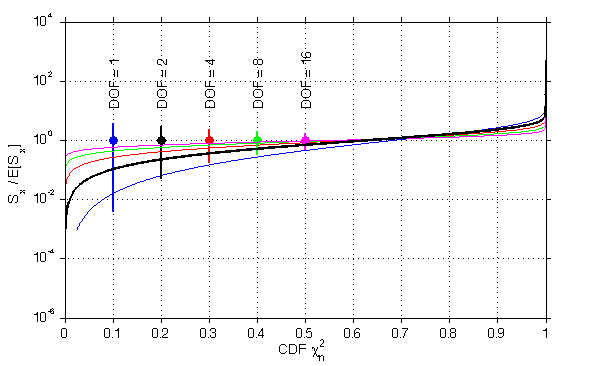
Plots of chi2 for these different degrees of freedom.
x = logspace(-3,3,1000);
jmkfigure(101,2,0.5);
clf
dof = [1 2 4 8 16];
nn = 0
col = {'b' 'k' 'r' 'g' 'm'}
for i=1:length(dof);
  nn = nn+1;
  pp = chi2cdf(x,dof(i));
  semilogy(pp,x/dof(i),'col',col{i},'linewi',1);
  hold on;
%  set(gca,'xlim',[1e-2 100]);
  grid on;
  ind = find(pp>0.05);ind = ind(1);
  ind2 = find(pp>0.95);ind2 = ind2(1);

  line(nn*0.1*[1 1],[x(ind)/dof(i) x(ind2)/dof(i)],'linewi',2,'col',col{i});
  plot(nn*0.1,1,'o','markersi',7,'markerfacecol',col{i},'linewi',2,'col',col{i});
  text(nn*0.1,10,sprintf('DOF = %d',dof(i)),'rotat',90);

%  line([0.01 100],[0.05 0.05]);
%  line([0.01 100],1-[0.05 0.05]);


end;
pp = chi2cdf(x,2);
semilogx(pp,x/2,'linewi',2);
ylabel('S_x / E[S_x]','fontsi',12);
xlabel('CDF \chi^2_n','fontsi',12);
if dop
  docprint('chi2','FftTechniques.m');
end;

% print -dpng -r150 doc/chi2
nn =

     0


col =

    'b'    'k'    'r'    'g'    'm'